Robotics |
| It studies the design, construction, operation and applications of robots. Estudia el diseño, construcción, operación y aplicación de los robots. |
End Effector |
| The device that is attached at the end of a robotic arm is called end effector. It is designed to interact with the objects in the environment and the environment itself. The figure below shows an end effector in three dimensions and in two dimensions. In the 3D robot of the figure, the end effector requires four variables to describe its position and orientation. In the 2D robot of the figure, the end effector requires only three variables to describe its position and orientation. El dispositivo que está sujetado al final de un arma de robot se llama efector final. Este está diseñado para interactuar con los objetos en el ambiente y el propio ambiente. La figura de abajo muestra un efector final en tres dimensiones y en dos dimensiones. En el robot de 3D de la figura, el efector final requiere cuatro variables para describir su posición y su orientación. En el robot de 2D de la figura, el efector final requiere solamente tres variables para describir su posición y su orientación. |
| Problem 1 |
| In the robot below, the orientation of the end effector is not important. Find the value of the angles B and C to set the position of the end effector at (a) x = 2.2 and y = 4.7, (b) x = -1.2 and y = 4.7. En el robot de abajo, la orientación del efector final no es importante. Encuentre el valor de los ángulos B y C para fijar la posición del efector final en (a) x = 2.2, y = 4.7, (b) x = -1.2, y = 4.7. |
| Problem 2 |
| Find the value of the angles α1, β1, α2, β2 to set the position of the end effector in x = 2.2 and y = 4.7. Encuentre el valor de los ángulos α1, β1, α2, β2 para fijar la posición del efector final en x = 2.2, y = 4.7. |
| Problem 3 |
| Find the value of the angles α1, β1, α2, β2 to set the position of the end effector in x = -1.2 and y = 4.7. Encuentre el valor de los ángulos α1, β1, α2, β2 para fijar la posición del efector final en x = -1.2, y = 4.7. |
| Problem 4 |
| Create a Wintempla dialog application called Robot to simulate the 2D Robot of the previous problem. Cree una aplicación de diálogo de Wintempla llamada Robot para simular el Robot de 2D del problema previo. |
| Step A |
| Add a Custom Control. From Microsoft Visual Studio menu Tools > Add Wintempla Item > Custom Control . Set the name to SimView and click the Add button. Agregue un Custom Control. Desde el menú de Microsoft Visual Studio Tools > Add Wintempla Item > Custom Control . Fije el nombre a SimView y de clic en el botón de Add. |
| Step B |
| Edit the GUI interface. From Microsoft Visual Studio menu Tools > Wintempla . Add six Textboxes, six Labels, two Sliders and a Custom Control (To see the Custom Control, click the green asterisk to display all the controls in the toolbox). After inserting the Custom Control, set the Class Name to SimView as shown. Edite la interface GUI. Desde el menú de Microsoft Visual Studio Tools > Wintempla Item . Fije el nombre a SimView y de clic en el botón de Add. Agregue seis Textboxes, seis Labels, dos Sliders y un Custom Control (para ver el Custom Control, haga clic en el asterisco verde para mostrar todos los controles en la caja de herramientas, toolbox). Después de insertar el Custom Control, fije la Class Name a SimView como se muestra. |
| Step C |
| Edit the files SimView.h and SimView.cpp. Edite los archivos SimView.h and SimView.cpp. |
| SimView.h |
| //____________________________________________________________ SimView.h #pragma once #include "resource.h" #define MAX_VALUE 6 //To create an object of this class, you must insert a Custom Control in the GUI class SimView: public Win::Window { public: SimView(); ~SimView(); Direct::Graphics graphics; Direct::SolidBrush brushGreen; Direct::SolidBrush brushBlue; D2D1_SIZE_F size; double x = 0.0f; double y = 0.0f; double x1= 0.0f; double y1 = 0.0f; double x2 = 0.0f; double y2 = 0.0f; float TransformX(double inx); float TransformY(double iny); //____________________________________________________ Font virtual void SetFont(Win::Gdi::Font& font); __declspec( property( put=SetFont) ) Win::Gdi::Font& Font; //____________________________________________________ Events bool IsEvent(Win::Event& e, int notification); private: const wchar_t * GetClassName(void){return L"SimView";} static bool isRegistered; protected: HFONT _hFont; //______ Wintempla GUI manager section begin: DO NOT EDIT AFTER THIS LINE void Window_Open(Win::Event& e); void Window_Paint(Win::Event& e); void Window_Size(Win::Event& e); }; |
| SimView.cpp |
| //____________________________________________________________ SimView.cpp #include "stdafx.h" #include "SimView.h" bool SimView::isRegistered= false; SimView::SimView() { if (!this->isRegistered) { this->RegisterClassEx( LoadCursor(NULL, IDC_ARROW), (HBRUSH)::GetStockObject(NULL_BRUSH)); this->isRegistered = true; } size.width = 0; size.height = 0; } SimView::~SimView() { } float SimView::TransformX(double inx) { return size.width*(float)inx/(2.0f*MAX_VALUE) + size.width/2.0f; } float SimView::TransformY(double iny) { return size.height*(float)iny/(-2.0f*MAX_VALUE) + size.height/2.0f; } void SimView::Window_Open(Win::Event& e) { brushGreen.Create(graphics, 0.0f, 1.0f, 0.0f, 1.0f); brushBlue.Create(graphics, 0.0f, 0.0f, 1.0f, 1.0f); } void SimView::Window_Paint(Win::Event& e) { D2D1_ELLIPSE ellipse; ellipse.point.x = TransformX(x); ellipse.point.y = TransformY(y); ellipse.radiusX = 10.0f; ellipse.radiusY = 10.0f; if (graphics.BeginDraw(hWnd, width, height, RGB(0, 0, 0)) == false) return; graphics.SetTransform(D2D1::Matrix3x2F::Identity()); graphics.DrawLine(TransformX(0.0), TransformY(0.0), TransformX(x1), TransformY(y1), brushBlue, 3.0f); graphics.DrawLine(TransformX(x1), TransformY(y1), TransformX(x2), TransformY(y2), brushBlue, 3.0f); graphics.FillEllipse(ellipse, brushGreen); graphics.EndDraw(true); } void SimView::Window_Size(Win::Event& e) { graphics.Resize(hWnd, width, height); size = graphics.GetSize(); } void SimView::SetFont(Win::Gdi::Font& font) { this->_hFont = font.GetHFONT(); ::InvalidateRect(hWnd, NULL, FALSE); } bool SimView::IsEvent(Win::Event& e, int notification) { if (e.uMsg!=WM_COMMAND) return false; const int id = LOWORD(e.wParam); const int notificationd = HIWORD(e.wParam); if (id != this->id) return false; if (notificationd!=notification) return false; return true; } |
| Step D |
| Edit the files Robot.h and Robot.cpp. Edite los archivos Robot.h and Robot.cpp. |
| Robot.h |
| #pragma once //______________________________________ Robot.h #include "Resource.h" #include "SimView.h" #define RESOLUTION 200 class Robot: public Win::Dialog { public: Robot() { } ~Robot() { } void RefreshView(); . . . }; |
| Robot.cpp |
| . . . void Robot::Window_Open(Win::Event& e) { //________________________________________________________ sldX sldX.SetRange(0, RESOLUTION); sldX.Position = RESOLUTION/2; tbxX.DoubleValue = 0.0; //________________________________________________________ sldY sldY.SetRange(0, RESOLUTION); sldY.Position = RESOLUTION/2; tbxY.DoubleValue = 0.0; } void Robot::sldX_Hscroll(Win::Event& e) { int position = 0; if (sldX.GetPosition(position) == false) return; tbxX.DoubleValue = 2.0*MAX_VALUE*(position/(double)RESOLUTION) - MAX_VALUE; RefreshView(); } void Robot::sldY_Hscroll(Win::Event& e) { int position = 0; if (sldY.GetPosition(position) == false) return; tbxY.DoubleValue = 2.0*MAX_VALUE*(position/(double)RESOLUTION) - MAX_VALUE; RefreshView(); } void Robot::RefreshView() { //________________________________________________ 1. Local variables const double x = tbxX.DoubleValue; const double y = tbxY.DoubleValue; const double a = 2.0; const double b = 4.0; //________________________________________________ 2. C and B const double c = sqrt(x*x + y*y); const double C = acos( (a*a + b*b - c*c)/(2.0*a*b)); const double B = acos( (a*a + c*c - b*b)/(2.0*a*c)); //________________________________________________ 3. alpha and beta double lambda = atan2(y, x); if (lambda < 0.0) lambda += (2.0*M_PI); const double alpha1 = lambda + B; const double alpha2 = lambda - B; double beta1 = atan2(y - a * sin(alpha1), x - a * cos(alpha1) ); double beta2 = atan2(y - a * sin(alpha2), x - a * cos(alpha2) ); if (beta1 < 0.0) beta1 += (2.0*M_PI); if (beta2 < 0.0) beta2 += (2.0*M_PI); //________________________________________________ 4. Display in GUI tbxBeta1.DoubleValue = beta1*180.0/M_PI; tbxBeta2.DoubleValue = beta2*180.0/M_PI; tbxAlpha1.DoubleValue = alpha1*180.0/M_PI; tbxAlpha2.DoubleValue = alpha2*180.0/M_PI; //________________________________________________ 5. Move bars customControlSim.x = x; customControlSim.y = y; // customControlSim.x1 = a*cos(alpha1); customControlSim.y1 = a*sin(alpha1); // customControlSim.x2 = customControlSim.x1 + b*cos(beta1); customControlSim.y2 = customControlSim.y1 + b*sin(beta1); // customControlSim.Repaint(NULL, false); } |
Optimization |
| It is possible to use optimization algorithms to find the values of θ1 and θ2 by defining an error function. Es posible usar algoritmos de optimización para encontrar los valores de θ1 y θ2 definiendo una función de error. |
| Problem 5 |
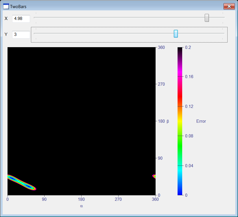
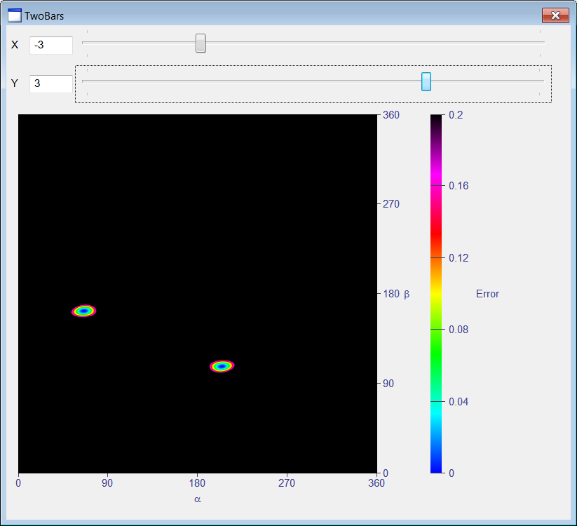
| Create a Wintempla dialog application called TwoBars to plot the error function shown below. After creating the project, use Wintempla to edit the GUI, click on "Show All Control in Toolbox" in the toolbar and insert a "Color Map" control to display the graph. Cree una aplicación de diálogo de Wintempla llamada TwoBars para graficar la función de error mostrada. Después de crear el proyecto, use Wintempla para editar la GUI, haga clic en "Show All Control in Toolbox" en la barra de herramientas e inserte un control de "Color Map" para mostrar la gráfica. |
| Step A |
| Edit the TwoBars.h file, do not forget to derivate the main class from Sys::IColorMapDataProvider. Edite el archivo TwoBars.h, no se olvide de derivar la clase principal desde Sys::IColorMapDataProvider. |
| TwoBars.h |
| #pragma once //______________________________________ TwoBars.h #include "Resource.h" class TwoBars: public Win::Dialog, public Sys::IColorMapDataProvider { public: TwoBars() { } ~TwoBars() { } double x = 0.0; double y = 0.0; protected: //_____________________________________________Sys::IColorMapDataProvider void GetDataRowZ(const int row, const int in_countX, const double* in_x, const double in_y, double* out_z); . . . }; |
| Step B |
| Edit the TwoBars.cpp file. Edite el archivo TwoBars.cpp. |
| TwoBars.cpp |
| . . . void TwoBars::Window_Open(Win::Event& e) { //________________________________________________________ mapError mapError.MinX = 0.0; mapError.MaxX = 360.0; mapError.MinY = 0.0; mapError.MaxY = 360.0; mapError.MinZ = 0.0; mapError.MaxZ = 0.2; mapError.SetPixelsResolutionX(512); mapError.SetPixelsResolutionY(512); mapError.SetCaptionX(L"a", true); mapError.SetCaptionY(L"b", true); mapError.SetCaptionZ(L"Error", false); mapError.SetDataProvider(this); //________________________________________________________ sldX sldX.SetRange(0, 200); sldX.Position = 50; //________________________________________________________ sldY sldY.SetRange(0, 200); sldY.Position = 50; // tbxX.DoubleValue = 0.0; tbxY.DoubleValue = 0.0; mapError.Refresh(); } void TwoBars::GetDataRowZ(const int row, const int in_countX, const double* in_x, const double in_y, double* out_z) { double alpha = 0.0; double beta = 0.0; double dx, dy; for (int i = 0; i < in_countX; i++) { alpha = in_x[i]*M_PI/180.0; beta = in_y*M_PI/180.0; dx = x - 2.0*cos(alpha) - 4.0*cos(beta); dy = y - 2.0*sin(alpha) - 4.0*sin(beta); out_z[i] = dx*dx + dy*dy; } } void TwoBars::sldX_Hscroll(Win::Event& e) { int position = 0; if (sldX.GetPosition(position) == false) return; x = 12.0*position/200.0 - 6.0; tbxX.DoubleValue = x; mapError.Refresh(); } void TwoBars::sldY_Hscroll(Win::Event& e) { int position = 0; if (sldY.GetPosition(position) == false) return; y = 12.0*position/200.0 - 6.0; tbxY.DoubleValue = y; mapError.Refresh(); } |
| Problem 6 |
| Create a Wintempla dialog application called BarSol to compute the optimization error for uniformly distributed values for θ1 and θ2. After creating the project, insert a multiline textbox to display the results. Also insert two textboxes, two labels and one button as shown below. One textbox is for the resolution and the other textbox is for the maximum error. Cree una aplicación de diálogo de Wintempla llamada BarSol para calcular el error de optimización para valores uniformemente distribuidos para θ1 y θ2. Después de crear el proyecto, inserte una caja multilínea para mostrar los resultados. También inserte dos cajas de texto, dos etiquetas y un botón cómo se muestra. Una caja de texto es para la resolución y la otra para el error máximo. |
| BarSol.cpp |
| . . . void BarSol::Window_Open(Win::Event& e) { tbxMaxError.DoubleValue = 0.01; tbxResolution.IntValue = 100; } void BarSol::btCompute_Click(Win::Event& e) { const double maxError = tbxMaxError.DoubleValue; wstring text = L"alpha\t\tbeta\t\terror\r\n"; wchar_t tmp[512]; const int resolution = tbxResolution.IntValue; const double delta = 360.0/resolution; double alpha, beta, error; double dx, dy; for (alpha = 0.0; alpha < 360.0; alpha += delta) { for (beta = 0.0; beta < 360.0; beta += delta) { dx = 5.0 - 2.0*cos(alpha*M_PI/180.0) - 4.0*cos(beta*M_PI/180.0); dy = 3.0 - 2.0*sin(alpha*M_PI/180.0) - 4.0*sin(beta*M_PI/180.0); error = dx*dx + dy*dy; if (error > maxError) continue; _snwprintf_s(tmp, 512, _TRUNCATE, L"%.4f\t\t%.4f\t\t%.4f\r\n", alpha, beta, error); text += tmp; } } tbxOutput.Text = text; } |
Artificial Neural Networks |
| In some cases, it is possible to use an artificial neural network to find the configuration of the robot using the desired position of the end effector. However, if the robot has two or more configurations to obtain one desired position of the end effector, an artificial neural network will NOT be able to learn multiple configurations. In fact, only one robot configuration for each position (and orientation) of the end effector can be included in the training set. En algunos casos, es posible usar una red neuronal artificial para encontrar la configuración de un robot usando la posición deseada del efector final. Sin embargo, si el robot tiene dos o más configuraciones para conseguir la posición deseada del efector final, una red neuronal artificial NO podrá aprender las dos configuraciones. De hecho, solamente una configuración del robot para cada posición (y orientación) del efector final puede ser incluida en el conjunto de datos de entrenamiento. |
| Problem 7 |
| Create a Wintempla dialog application called BuildTrainSet to create a dataset to train an artificial neural network to compute the values of α and β for a given position of the end effector in the figure. After creating the project, edit the GUI as shown below. Cree una aplicación de diálogo de Wintempla llamada BuildTrainSet para crear un conjunto de datos para entrenar una red neuronal artificial para calcular los valores de α y β para una posición dada del efector final de la figura. Después de crear el proyecto, edite la GUI cómo se muestra debajo. |
| Step A |
| Edit the BuildTrainSet.cpp file as shown. Edite el archivo BuilTrainSet.cpp cómo se muestra. |
| BuilTrainSet.cpp |
| . . . void BuildTrainSet::btBuild_Click(Win::Event& e) { //____________________________________________________ 1. Prompt user for filename Win::FileDlg dlg; dlg.Clear(); dlg.SetFilter(L"Comma separated values (*.csv)\0*.csv\0\0", 0, L"csv"); if (dlg.BeginDialog(hWnd, L"Save", true) != TRUE) return; //____________________________________________________ 2. Create file Sys::File file; if (file.CreateForWritting(dlg.GetFileNameFullPath()) == false) { Sys::DisplayLastError(hWnd, L"Saving CSV file"); return; } //____________________________________________________ 3. Write file const int resolution = tbxResolution.IntValue; const double delta = 180.0/resolution; double alpha, beta, radAlpha, radBeta; double x, y; char text[512]; _snprintf_s(text, 512, _TRUNCATE, "x, y, alpha, beta\r\n"); file.WriteText(text); for (alpha = 0.0; alpha < 180.0; alpha += delta) { radAlpha = alpha*M_PI/180.0; for (beta = alpha + delta; beta < 180.0; beta += delta) { radBeta = beta*M_PI/180.0; x = 2.0*cos(radAlpha) + 4.0*cos(radBeta); y = 2.0*sin(radAlpha) + 4.0*sin(radBeta); _snprintf_s(text, 512, _TRUNCATE, "%.7f, %.7f, %.7f, %.7f\r\n", x, y, alpha, beta); file.WriteText(text); } } } |
| Step B |
| From Microsoft Visual Studio menu Build > Configuration Manager change the configuration to "Release". Then, compile and run the program. Desde el menú de Microsoft Visual Studio Build > Configuration Manager cambie la configuración a "Release". Entonces, compile y ejecute el programa. |
| Step C |
| Set the resolution to 180 (180/180=1 degrees), then create a filename called dataset.csv as shown. Fije la resolución a 180 (180/180=1 grados), entonces cree un archivo llamado dataset.csv cómo se muestra. |
| Problem 8 |
| Use Neural Lab (4.5 or later) to create a project called Inverse, select the option "Main file only". After creating the project, copy the dataset.csv file to the Inverse folder as shown. Edit the Main.lab file to create the training set input and the training set target for α and for β. Use Neural Lab (4.5 o posterior) para crear un proyecto llamado Inverse, seleccione la opción de "Main file only". Después de crear el proyecto, copie el archivo dataset.csv a la carpeta del proyecto Inverse como se muestra. Edite el archivo Main.lab para crear la entrada del conjunto de entrenamiento y la meta del conjunto de datos de entrenamiento para α y para β. |

| Inverse\Main.lab |
| //_______________________________________ 1. Load dataset Matrix dataset; dataset.Load(); //_______________________________________ 2. Train set input Vector index; index.Create(2); index[0] = 0; index[1] = 1; Matrix trainSetInput = dataset.GetCols(index); trainSetInput.Save(); //_______________________________________ 3. alpha Matrix alpha = dataset.GetCol(2); alpha.Save(); //_______________________________________ 4. beta Matrix beta = dataset.GetCol(3); beta.Save(); |
| Step A |
| Add a file called TrainAlpha.lab as shown below to train an artificial neural network to estimate the value of α. After editing the file, execute the code to train the artificial neural network for α. Agregue un archivo llamado TrainAlpha.lab cómo se muestra debajo para entrenar una red neuronal artificial para estimar el valor de α. Después de editar el archivo, ejecute el código para entrenar la red neuronal artificial para α. |
| Inverse\TrainAlpha.lab |
| //_______________________________________ 1. Network setup DeepNet netAlpha; netAlpha.Create(2, 2); netAlpha.SetLayer(0, 1, 20); netAlpha.SetLayer(1, 1, 1); //_______________________________________ 2. Input scaling netAlpha.SetInScaler(0, -6.0, 6.0); // x netAlpha.SetInScaler(1, 0.0, 6.0); // y //_______________________________________ 3. Output scaling netAlpha.SetOutScaler(0, 0.0, 179.0); //_______________________________________ 4. Training set Matrix trainSetInput; trainSetInput.Load(); Matrix alpha; alpha.Load(); netAlpha.SetTrainSet(trainSetInput, alpha, false); //_______________________________________ 5. Train using simulated annealing netAlpha.TrainSimAnneal( 20, //Number of Temperatures 20, //Number Iterations 15, //Initial Temperature 0.001, //Final Temperature true, //Is Cooling Schedule Linear? 2, //Number of Cycles 1.0e-5, //Goal (desired mse) true //Use Singular Value Decomposition ); //_______________________________________ 6. Train using conjugate gradient netAlpha.TrainConjGrad(2500, 1.0e-8); //_______________________________________ 7. Save the trained network netAlpha.Save(); |
| Step B |
| Add a file called TrainBeta.lab as shown below to train an artificial neural network to estimate the value of β. After editing the file, execute the code. Agregue un archivo llamado TrainBeta.lab cómo se muestra debajo para entrenar una red neuronal artificial para estimar el valor de β. Después de editar el archivo, ejecute el código. |
| Inverse\TrainBeta.lab |
| //_______________________________________ 1. Network setup DeepNet netBeta; netBeta.Create(2, 2); netBeta.SetLayer(0, 1, 20); netBeta.SetLayer(1, 1, 1); //_______________________________________ 2. Input scaling netBeta.SetInScaler(0, -6.0, 6.0); // x netBeta.SetInScaler(1, 0.0, 6.0); // y //_______________________________________ 3. Output scaling netBeta.SetOutScaler(0, 0.0, 179.0); //_______________________________________ 4. Training set Matrix trainSetInput; trainSetInput.Load(); Matrix beta; beta.Load(); netBeta.SetTrainSet(trainSetInput, beta, false); //_______________________________________ 5. Train using simulated annealing netBeta.TrainSimAnneal( 20, //Number of Temperatures 20, //Number Iterations 15, //Initial Temperature 0.001, //Final Temperature true, //Is Cooling Schedule Linear? 2, //Number of Cycles 1.0e-5, //Goal (desired mse) true //Use Singular Value Decomposition ); //_______________________________________ 6. Train using conjugate gradient netBeta.TrainConjGrad(2500, 1.0e-8); //_______________________________________ 7. Save the trained network netBeta.Save(); |
| Step C |
| Add a file called Test.lab to evaluate the performance of the artificial neural network. Agregue un archivo llamado Test.lab para evaluar el desempeño de la red neuronal artificial. |
| Inverse\Test.lab |
| //_______________________________________ 1. Load networks DeepNet netAlpha; netAlpha.Load(); DeepNet netBeta; netBeta.Load(); //_______________________________________ 2. Input Matrix trainSetInput; trainSetInput.Load(); int count = trainSetInput.GetRowCount(); Vector index; index.CreateRandomSet(100, count-1); Matrix inputXY = trainSetInput.GetRows(index); //_______________________________________ 3. Run networks Matrix alpha; netAlpha.Run(inputXY, alpha); Matrix beta; netBeta.Run(inputXY, beta); //_______________________________________ 4. Compute x and y Matrix radAlpha = alpha*3.1416/180.0; Matrix radBeta = beta*3.1416/180.0; Matrix x = 2.0*cos(radAlpha) + 4.0*cos(radBeta); Matrix y = 2.0*sin(radAlpha) + 4.0*sin(radBeta); //_______________________________________ 5. Plot target XyChart xyGraph; xyGraph.SetColorMode(2); xyGraph.SetLimits(-6.0, 6.0, 0.0, 6.0); Vector vx = inputXY.GetColVec(0); Vector vy = inputXY.GetColVec(1); xyGraph.AddGraph(vx, vy, "Target", 1, 2, 0, 100, 255); //_______________________________________ 6. Plot ANN results; vx = x.GetColVec(0); vy = y.GetColVec(0); xyGraph.AddGraph(vx, vy, "ANN", 1, 3, 0, 255, 0); xyGraph.SaveAndShow(); xyGraph.SavePDF(0.0); |
Frame of reference |
| In robotics, physics and other areas, it is very important to have point in space and time for reference. This point is called Frame of Reference and it is depicted as shown below. En robótica, física y otras áreas, es muy importante tener un punto en espacio y tiempo para referencia. Este punto es llamado Marco de Referencia y se dibuja como se muestra debajo. |
Joints |
| There are two types of joints: rotational joints and prismatic joints (extending). A joint connects two different frames. The joint allows to change the distance or rotation angle between two frames. Hay dos tipos de uniones: uniones de rotación y uniones prismáticas (extendedoras). Una unión conecta dos frames diferentes. La unión permite cambiar la distancia o el ángulo de rotación entre dos frames. |
Joint Variable |
| Each join has a parameter associated with the joint. A prismatic joint has a variable to represent the distance between the two frames. A rotational joint has a variable to represent the angle between the two frames. Cada unión tiene un parámetro asociado con la unión. Una unión prismática tiene una variable para representar la distancia entre las dos frames. Una unión de rotación tiene una variable para representar el ángulo entre las dos frames. |
Homogeneous Transformation Matrix |
| It allows transforming the coordinates of a point relative to one frame to the coordinates relative to another frame. This matrix is very useful in robotics to know the position of any part of the robot relative to the base frame. An homogeneous transformation matrix has four rows and four columns. The last row of the matrix is composed of three "zeros" and one "one" as shown in the figure. The matrix includes inside a rotation matrix and a displacement vector. An homogeneous transformation matrix has a superscript to indicate the current frame, and a subscript to indicate the next frame. In the example, both frames are separated a distance of two in the X direction. Esta permite transformar las coordenadas de un punto relativas a una frame a las coordenadas relativas a otra frame. Esta matriz es muy útil en robótica para conocer la posición de cualquier parte del robot en forma relativa a la frame base. Una matriz de transformación homogénea tiene cuatro renglones y cuatro columnas. El último renglón de la matriz está compuesto de tres "ceros" y un "uno" como se muestra en la figura. La matriz incluye dentro una matriz de rotación y un vector de desplazamiento. Una matriz de transformación homogénea tiene un superíndice para indicar la frame actual, y un subíndice para indicar la frame siguiente. En el ejemplo, ambas frames están separadas una distancia de dos en la dirección de X. |
Point Transformation |
| In the figure below, there is the point P. The point P does not change position, but the point P can be expressed using as reference frame 1 or frame 2. P1 denotes the point P relative to frame 1, while P2 denotes the point P relative to frame 2. Observe that in this type of notation, the point is expressed by a vector column with four elements. Observe also that the value in the last row of this vector is always one. The figure below shows the value of P2. The figure also illustrates how compute the value of P1, that is, the value P relative to Frame 1. Thus, once the homogeneous transformation matrix between two frames has been computed, it is possible to transform a point from one frame to the other frame. En la figura de abajo, está el punto P. El punto P no cambia de posición, pero el punto P puede ser expresado usando como referencia la frame 1 o la frame 2. P1 denota el punto P en forma relativa con la frame 1, mientras P2 denota el punto P en forma relativa con la frame 2. Observe que en este tipo de notación, el punto se expresa por un vector columna con cuatro renglones. Observe también que el valor en el último renglón de este vector es siempre uno. La figura de abajo muestra el valor de P2. La figura también ilustra cómo calcular el valor de P1, esto es, el valor de P en forma relativa a la frame 1. Así, una vez que la matriz de transformación homogénea entre dos frames sea calculado, es posible transformar un punto de una frame a la otra frame. |
| Problem 9 |
| Compute the homogeneous transformation matrix for the system below. Calcule la matriz de transformación homogénea para el sistema debajo. |
| Problem 10 |
| Compute the homogeneous transformation matrix for the system below. Calcule la matriz de transformación homogénea para el sistema debajo. |
| Problem 11 |
| Compute the homogeneous transformation matrix for the system below. Calcule la matriz de transformación homogénea para el sistema debajo. |
| Tip |
| The figure below shows the formulas for rotation around each axis for a left-handed coordinate system and a right-handed coordinate system. La figura de abajo muestra las fórmulas para rotación alrededor de cada eje para un sistema de coordenadas de mano derecha y para un sistema de coordenadas de mano izquierda. |
| Problem 12 |
| Compute the homogeneous transformation matrix for the system below for a right-handed coordinate system. Calcule la matriz de transformación homogénea para el sistema debajo para un sistema de coordenadas de mano derecha. |
Denavit-Hartenberg |
The method of Denavit-Hartenberg allows computing the homogeneous transformation matrix using an alternative method. This method includes some rules, they are called frame rules and are:
El método de Denavit-Hartenberg permite calcular la matriz de transformación homogénea usando un método alternativo. Este método incluye algunas reglas, estas son llamadas las reglas de las frames y son:
|
Denavit-Hartenberg parameters |
| The method of Denavit-Hartenberg has four input parameters: θ, α, r and d Once these parameters have been computed, the formula below is used to compute the homogeneous transformation matrix. Wintempla provides the function Math::Oper::Denavit to compute this matrix. El método de Denavit-Hartenberg tiene cuatro parámetros de entrada: θ, α, r y d. Una vez que estos parámetros han sido calculados, la fórmula de abajo se usa para calcular la matriz de transformación homogénea. Wintempla proporciona la función Math::Oper::Denavit para calcular esta matriz. |
Computation of θ |
| θ is the amount of rotation around the Zn-1 axis to get axis Xn-1 to match the direction of Xn axis as shown in the figure below. θ es la cantidad de rotación alrededor del eje Zn-1 para que el eje Xn-1 tenga la misma dirección del eje Xn como se muestra en la figura. |
Computation of α |
| α is the amount of rotation around the Xn axis to get the axis Zn-1 to match the direction of Zn axis as shown in the figure below. α es la cantidad de rotación alrededor del eje Xn para que el eje Zn-1 tenga la misma dirección que el eje Zn como se muestra en la figura. |
Computation of r |
| r is the displacement along the Xn axis between the center of frame n-1 and the center of frame n as shown in the figure below. r es la desplazamiento a lo largo del eje Xn entre el centro de la frame n-1 y el centro de la frame n como se muestra en la figura. |
Computation of d |
| d is the distance between the centers of the two frames in the direction of the Zn-1 axis as shown in the figure below. d es la distancia entre los centros de las dos frames en la dirección del eje Zn-1 como se muestra en la figura. |
| Problem 13 |
| Compute the Denavit-Hartenberg parameters for the system shown. Calcule los parámetros de Denavit-Hartenberg para el sistema mostrado. |
| Problem 14 |
| Compute the Denavit-Hartenberg parameters for the system shown. Calcule los parámetros de Denavit-Hartenberg para el sistema mostrado. |
| Problem 15 |
| Compute the Denavit-Hartenberg parameters for the system shown. Calcule los parámetros de Denavit-Hartenberg para el sistema mostrado. |
| Problem 16 |
| Compute the Denavit-Hartenberg parameters for the system shown. Calcule los parámetros de Denavit-Hartenberg para el sistema mostrado. |
| Problem 17 |
| Compute the Denavit-Hartenberg parameters for the system shown. Calcule los parámetros de Denavit-Hartenberg para el sistema mostrado. |
| Problem 18 |
Create a DirectX application called Cartesian using Wintempla to test the cartesian manipulator. Press the
Cree una aplicación de DirectX llamada Cartesian usando Wintempla para probar el manipulador cartesiano. Presiona la tecla
|
| Step 1 |
| Edit the files Manipulator.h and Manipulator.cpp. Edite los archivos Manipulator.h and Manipulator.cpp. |
| Manipulator.h |
| #pragma once class Manipulator : public DX11::ColorVertexBuffer { public: Manipulator(); ~Manipulator(); DirectX::XMMATRIX world; void ChangeD1(ID3D11DeviceContext* deviceContext, double delta); void ChangeD2(ID3D11DeviceContext* deviceContext, double delta); void ChangeD3(ID3D11DeviceContext* deviceContext, double delta); void Turn(Sys::Stopwatch& stopWatch); private: MATRIX H01; MATRIX H12; MATRIX H23; MATRIX H02; MATRIX H03; double d1 = 0.0; double d2 = 0.0; double d3 = 0.0; void ComputeH(); FLOAT angleY = (FLOAT)0.0f; }; |
| Manipulato.cpp |
| . . . Manipulator::Manipulator() { world = DirectX::XMMatrixIdentity(); if (Setup(6, 6, D3D11_USAGE_DYNAMIC, D3D_PRIMITIVE_TOPOLOGY_LINELIST) == false) return; for (size_t i = 0; i < 6; i++) { vertex[i].position = DirectX::XMFLOAT3(0.0f, 0.0f, 0.0f); index[i] = i; } //_________________________________________________ Link 1 (Red) vertex[0].color = DirectX::XMFLOAT4(1.0f, 0.0f, 0.0f, 1.0f); vertex[1].color = DirectX::XMFLOAT4(1.0f, 0.0f, 0.0f, 1.0f); //_________________________________________________ Link 2 (Green) vertex[2].color = DirectX::XMFLOAT4(0.0f, 1.0f, 0.0f, 1.0f); vertex[3].color = DirectX::XMFLOAT4(0.0f, 1.0f, 0.0f, 1.0f); //_________________________________________________ Link 3 (Blue) vertex[4].color = DirectX::XMFLOAT4(0.0f, 0.0f, 1.0f, 1.0f); vertex[5].color = DirectX::XMFLOAT4(0.0f, 0.0f, 1.0f, 1.0f); ComputeH(); } Manipulator::~Manipulator() { } void Manipulator::ChangeD1(ID3D11DeviceContext* deviceContext, double delta) { d1 += delta; ComputeH(); this->DynamicUpdate(deviceContext, true, false); } void Manipulator::ChangeD2(ID3D11DeviceContext* deviceContext, double delta) { d2 += delta; ComputeH(); this->DynamicUpdate(deviceContext, true, false); } void Manipulator::ChangeD3(ID3D11DeviceContext* deviceContext, double delta) { d3 += delta; ComputeH(); this->DynamicUpdate(deviceContext, true, false); } void Manipulator::ComputeH() { Math::Oper::DenavitD(90.0, 90.0, 0.0, 4.0+d1, H01); Math::Oper::DenavitD(90.0, -90.0, 0.0, 8.0+d2, H12); Math::Oper::DenavitD(0.0, 0.0, 0.0, 5.0+d3, H23); Math::Oper::Product(H01, H12, H02); // H02 = H01*H12 Math::Oper::Product(H02, H23, H03); // H03 = H02*H23 // if (this->GetVertexCount() == 0) return; //_________________________________________________ Link 1 vertex[0].position = DirectX::XMFLOAT3(0.0f, 0.0f, 0.0f); vertex[1].position = DX11::Geometry::HomegeneousTransformation(H01, 0.0f, 0.0f, 0.0f); //_________________________________________________ Link 2 vertex[2].position = vertex[1].position; vertex[3].position = DX11::Geometry::HomegeneousTransformation(H02, 0.0f, 0.0f, 0.0f); //_________________________________________________ Link 3 vertex[4].position = vertex[3].position; vertex[5].position = DX11::Geometry::HomegeneousTransformation(H03, 0.0f, 0.0f, 0.0f); } void Manipulator::Turn(Sys::Stopwatch& stopWatch) { const FLOAT delta = (FLOAT)stopWatch.GetSeconds(); //________________________________________________________ 1. Rotate, translate and scale angleY += (0.5f*delta); world = DirectX::XMMatrixRotationY(angleY); if (angleY > DirectX::XM_2PI) angleY -= DirectX::XM_2PI; } |
| Step 2 |
| Edit the files Cartesian.h and Cartesian.cpp. Edite los archivos Cartesian.h and Cartesian.cpp. |
| Cartesian.h |
| #pragma once //______________________________________ Cartesian.h #include "Resource.h" #include "Manipulator.h" class Cartesian: public DX11::Window { public: Cartesian() { } ~Cartesian() { } //____________________________________________________ 1. Application Manipulator manipulator; . . . }; |
| Cartesian.cpp |
| . . . void Cartesian::Window_Open(Win::Event& e) { . . . //________________________________________________________________ 4. Setup the camera camera.position.x = 0.0f; camera.position.y = 2.0f; camera.position.z = -10.0f; // camera.lookAt.x = 0.0f; camera.lookAt.y = -0.2f; camera.lookAt.z = 1.0f; // camera.SetViewInfo(modeDesc.Width, modeDesc.Height, false); // Left-Handed coordinate system //________________________________________________________________ 5. Setup the application objects manipulator.Create(hWnd, device); } void Cartesian::RenderScene() { //________________________________________________ 1. Clear screen and camera update Clear(0.0f, 0.0f, 0.2f, 1.0f); camera.Update(); //________________________________________________ 2. Application objects manipulator.DynamicUpdate(deviceContext, true, false); manipulator.Render(deviceContext); if (keyboard[VK_SPACE]) manipulator.Turn(stopWatch); colorShader.Render(deviceContext, manipulator.GetIndexCount(), manipulator.world, camera); } void Cartesian::Window_KeyDown(Win::Event& e) { if (e.wParam>255) return; keyboard[e.wParam] =true; if (e.wParam == VK_ESCAPE) { if (isFullScreen) { ::DestroyWindow(hWnd); } else { if (::MessageBox(hWnd, L"Do you want to close?", L"Cartesian", MB_YESNO | MB_ICONQUESTION) == IDYES) ::DestroyWindow(hWnd); } } else if (e.wParam == '1') { manipulator.ChangeD1(deviceContext, 0.1); } else if (e.wParam == '2') { manipulator.ChangeD2(deviceContext, 0.1); } else if (e.wParam == '3') { manipulator.ChangeD3(deviceContext, 0.1); } else if (e.wParam == 'Q') { manipulator.ChangeD1(deviceContext, -0.1); } else if (e.wParam == 'W') { manipulator.ChangeD2(deviceContext, -0.1); } else if (e.wParam == 'E') { manipulator.ChangeD3(deviceContext, -0.1); } } . . . |
| Problem 19 |
| Create a DirectX application called Spherical using Wintempla to test the spherical manipulator. After creating the project, add a new class called Manipulator. Cree una aplicación de DirectX llamada Spherical usando Wintempla para probar el manipulador esférico. Después de crear el proyecto, agrega una nueva clase llamada Manipulator. |